Augmented Dickey–Fuller test (ADF & ADF TD)

An indicator that determines the stationarity of a price series.

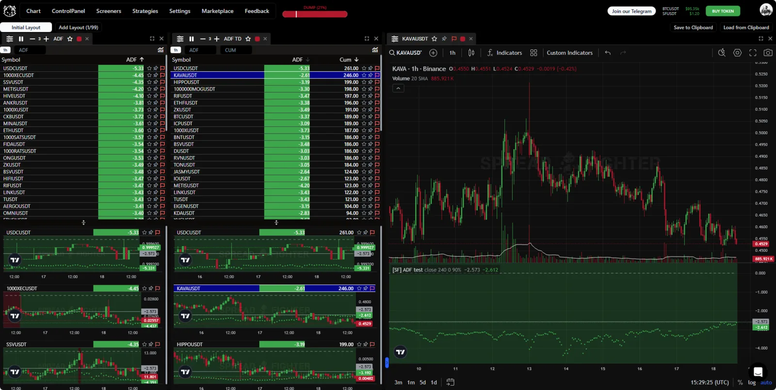
Indicator appearance.

Description

Model history

The Augmented Dickey–Fuller test (ADF test) is a statistical test used to check for a unit root in an autoregressive model and so to determine the stationarity of a time series. In financial markets it is widely used to analyze asset price series.

The test was developed and described by the British statisticians David Dickey and Wayne Fuller in 1979. The augmented version (ADF) was proposed to improve accuracy and reliability compared with the original Dickey–Fuller test.

What the model is used for in financial markets

1. Stationarity check: the ADF test is used to determine whether a time series is stationary or trending (that is, contains a unit root). Stationarity matters in time series modeling and econometric analysis, because many methods require stationary data.
2. Integration analysis: it is most often used in cointegration analysis, where multivariate time series are examined for long-term relationships.
3. Algorithmic trading decisions: a stationarity check helps develop strategies based on time series, including pairs trading and time series forecasting.

Why the augmented version is better than the plain one

1. Accounting for autocorrelation: the ADF test adds extra lags of the differences of the dependent variable to the model to account for high autocorrelation in time series data. This makes the test more reliable and accurate.
2. Flexibility: the augmented version can account for both random walks and deterministic trends, including a linear trend, in model estimation.
3. Fewer autocorrelated residuals: the ADF test corrects the problem of residual autocorrelation, which can distort results in the original Dickey–Fuller test.

https://en.wikipedia.org/wiki/Dickey%E2%80%93Fuller_test

Functionality

Widgets

The ADF model has 2 widget variants: ADF and ADF Time Dominance.

• ADF calculates the Dickey–Fuller test statistic and ranks assets with the minimum/maximum ADF value.
• ADF TD calculates the time in minutes during which the asset stayed stationary and ranks assets with the longest period of stationarity.

The data goes into a table with these columns:

• ADF - the Dickey–Fuller test statistic.
• Cum - the number of minutes during which the asset was stationary.

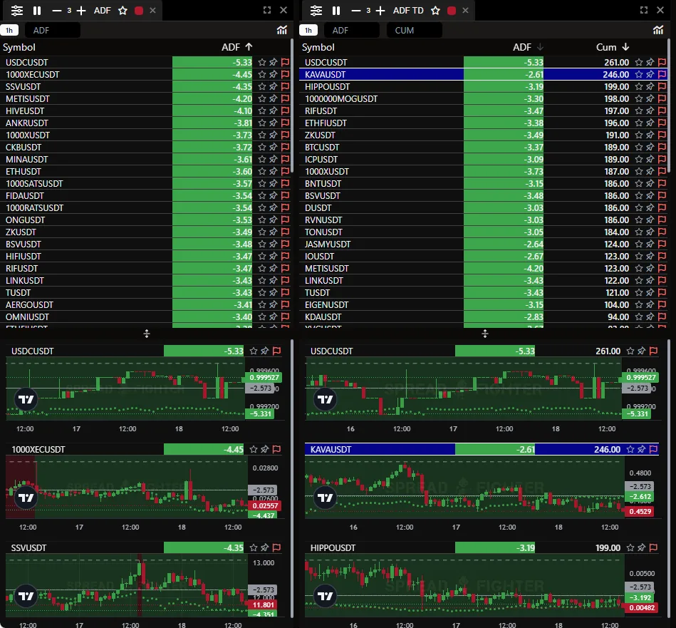
ADF widgets.

Indicator

The indicator runs the Dickey–Fuller test on the price series of the asset open on the chart. A green indicator color means the asset is stationary.

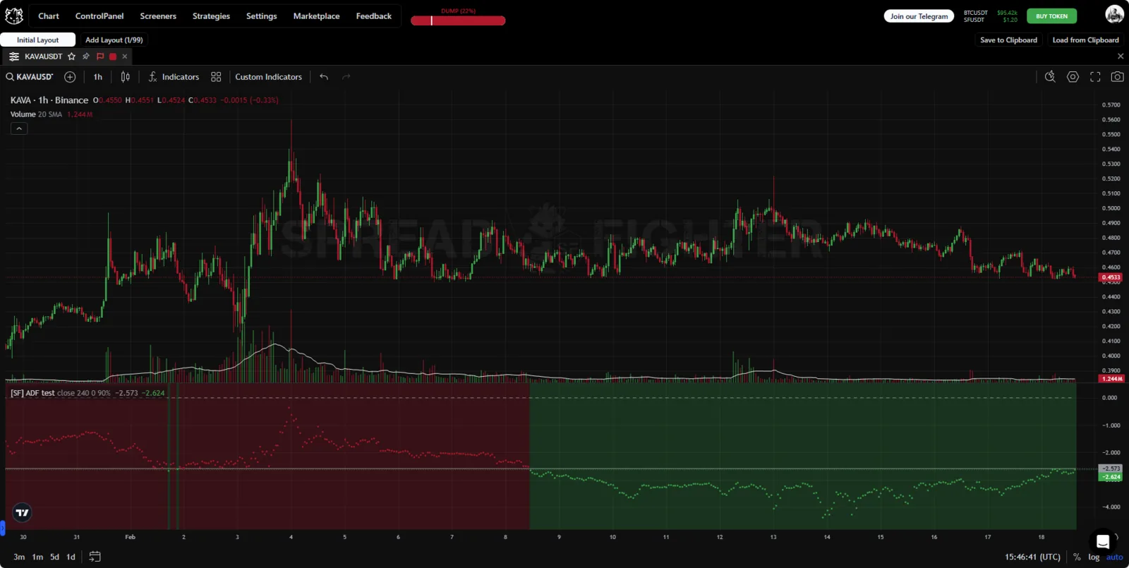
ADF indicator.

Use cases

The Augmented Dickey–Fuller test is widely used in quasi-arbitrage, pairs trading and basket trading to find cointegrated pairs.

tip

Cointegration is a property where a price series made of several non-stationary series, taken in a certain proportion, starts to become stationary.

Let us look at cointegration in a practical example.

BAT is an Ethereum token that supports the blockchain-based digital advertising platform of Brave Software. Internet users who browse with the free Brave web browser (available at Brave.com) can replace the ads they see with ads from the Brave ad network. Users then receive BAT from advertisers as compensation for their attention.

Source: Coinbase

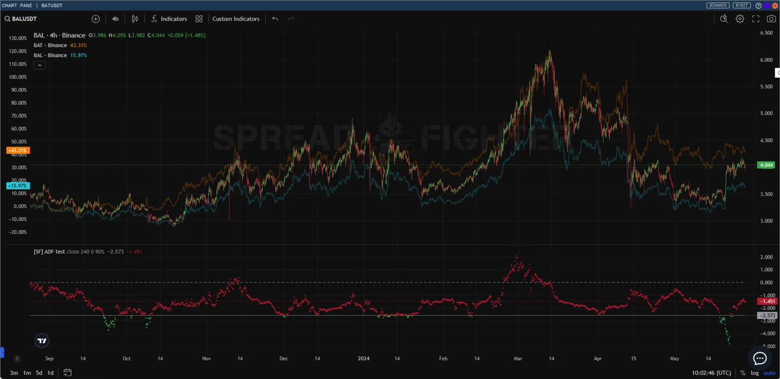
The BAT price series is not stationary.

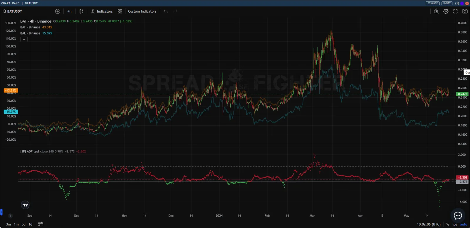
BAT

Balancer (BAL) is an Ethereum token behind the Balancer protocol. The protocol works as an automated market maker, so anyone can create trading pools and add liquidity to them, earning customizable trading fees. A Balancer pool can hold up to 8 tokens. Each token can have its own weight, which can be limited to as little as 2% of the total.

Source: Coinbase

The BAL price series, like BAT, is not stationary.

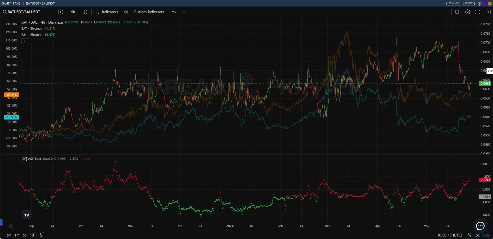
However, if you take a basket of BAT against BAL (BINANCE:BATUSDT/BINANCE:BALUSDT), the synthetic series starts to show stationarity over a certain period.

Trading stationary series has several advantages:

1. Predictability:
   • Less chance of sudden changes: stationary assets have stable statistical properties (mean, variance) over time, which makes their future values more predictable.
   • Historical data matters: since the parameters do not change over time, past data can be used to forecast future prices.
2. A defined structure:
   • Mean reversion: stationary assets tend to return to a long-term mean, which lets traders use strategies based on this principle (for example, pairs trading).
   • Some autocorrelation: stationary assets can show patterns in price changes, which allows building more accurate forecasting models.
3. Simple modeling and analysis:
   • Fewer difficulties in model estimation: for stationary assets you can use simple time series models, such as ARIMA (autoregressive integrated moving average), for analysis and forecasting.
   • Stable parameters: the parameters of models built on stationary data stay stable over time, which raises the reliability and accuracy of forecasts.
4. Lower risk:
   • Controllable risks: since stationary assets are less prone to extreme swings, traders can assess and manage risks more precisely.
   • Lower volatility: stable volatility makes trading more predictable and less stressful.
5. Arbitrage strategy opportunities:
   • Cointegration: when two or more stationary assets are cointegrated, traders can use an arbitrage strategy to profit from price imbalances.
   • Less dependence on trends: stationary assets offer more opportunities to trade reversions than trending markets do, which diversifies trading strategies.
6. Spotting seasonal and cyclical changes:
   • Pattern detection: using stationary variables helps find patterns, such as seasonal or cyclical changes, which can help develop trading strategies.
7. Efficient capital management:
   • Better data-driven decisions: thanks to the predictability and stability of stationary assets, traders can make better-founded decisions on capital management and position sizing.

In the end, trading stationary assets lets traders use the statistical properties of time series to build predictable, manageable and less risky trading strategies.

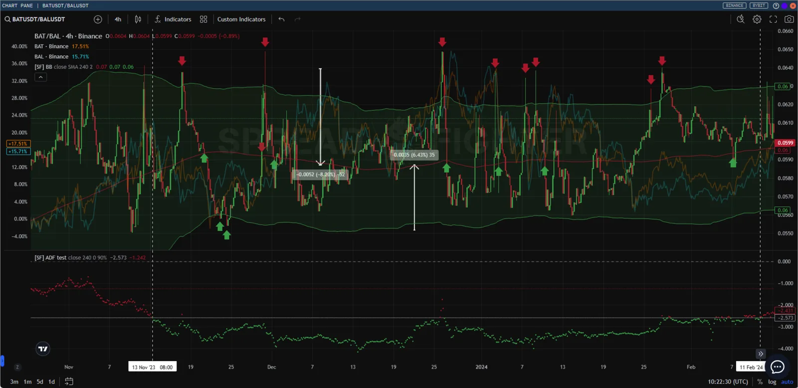
Example of the simplest trading logic for a synthetic stationary series.

But do not treat quasi-arbitrage of stationary series as a Holy Grail. Like any speculative activity, statistical arbitrage comes with a number of risks and tasks the trader has to solve.

1. The first problem is finding related assets. For example, if the crypto market is flat, classic cointegration tests can find quite a lot of related assets. But if Bitcoin starts a trending move up or down, it quickly turns out that the relationship is not that good, and the word hedge starts to lose its meaning along with the trader's deposit.
2. From this, and not only from this, follows the second problem: detecting a cointegration break in time, that is, a loss of the link between assets.
3. The third problem is finding the mean price, because there are many methods to determine it. All of them give different results.
4. The fourth problem is finding the entry point. Usually, standard deviations from the volume-weighted fair price are used. However, deviations can be calculated in different ways.
5. The fifth problem is a lack of infrastructure and software that lets you set risk or profit limits. And in general, software that makes it convenient to trade and select assets. Still, despite these problems, even the simplest interfaces and trading in this direction give a clear edge over most traders with the classic approach.