Liquidation Heatmap
A second way to display the same model as Liquidation Map. The map shows a forecast for the next few minutes around price and does not remember the past. The heatmap accumulates these forecasts on a fixed price grid and clears whatever price has already reached, leaving the fuel that has not been spent.
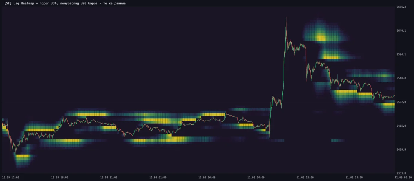
ETHUSDT, 10–11 September 2026. The bands stay at their prices while price moves away; the dark funnel along the track is what has already been spent. The yellow patch above price after the 11 September spike is a $109.8M cascade.
What it is
The heatmap is drawn over the candles and is fed by the same data series as Liquidation Map: the same model, the same widths, a different way of displaying it.
Every minute the model gives the density of expected liquidations around price. The map shows only the fresh one: the cloud follows price. The heatmap lays out each minute's density on a fixed price grid, ages the accumulated values with a half-life, and clears a cell on the same bar where price touched it. What stays on screen is not a forecast an hour ahead, but what the model pointed to many times in a row and where price has not been yet.
Hence the characteristic picture: a dark funnel along the price path and bright bands off to the side of it.
How it differs from Liquidation Map
| Liquidation Map | Liquidation Heatmap | |
|---|---|---|
| What it shows | A forecast for the horizon ahead of the current minute | Forecasts accumulated over the last hours minus what price has passed through |
| Geometry | A cloud around price, moving with it | Horizontal bands at fixed prices |
| Color | Red down, green up: who gets wiped out | One intensity scale, the eye reads the side |
| Memory | None | Yes, with a half-life |
The two indicators don't replace each other and live together on one chart. The map answers "where is volume expected right now and how far to place the stop". The heatmap answers "where did the model point over the last hours and what of that is not yet used up".
How to read it
Brightness is the model's accumulated attention, not dollars. The scale is relative: the brightest cell on screen is taken as one. You cannot compare brightness between instruments or between distant parts of the chart.
The dark funnel along price is not a hole in the data. It is spent fuel. The rule "a level disappears on touch" is the only thing we took from other people's accumulation maps, and the only one from that family that survived testing.
The bands stay in place. The grid is tied to prices, not to the screen: while price moves inside the window, the band boundaries don't move, and a level can be read off the price scale.
Once every few hours a transparent one-bar column appears. This is a grid shift: when price moves away from the center of the window by more than a third of its width, the anchor is moved, and the shift bar is cleared on purpose, otherwise a diagonal would appear in its place.
What is measured and what is not
This matters more than everything else on the page, so no softening.
The heatmap does not show price direction, just like Liquidation Map. Refuted on 20 instruments and three folds: the spread of the extreme deciles of the predicted side is −3.84 bp with a standard error of 8.52, t = −0.45. A bright band above means "if the move happens up, this many shorts will be wiped out", not "it will go up".
The +12.31 pp gain is about the model, not about this way of displaying it. The figure was measured on the forecast heatmap, that is, on Liquidation Map. Accumulation by itself was not measured as a predictor: the heatmap is a visualization of the same model, and it has no right to automatically take its figures as its own.
Open interest is not part of the model, and this was tested, not overlooked. Accumulation maps by ΔOI with leverage buckets, which is how other products of this class are built, capture 30–35% of the next hour's liquidation volume against 62% for a simple band around price. The contribution of OI on top of uniform inputs is +0.016 with an MDE of 0.029, that is, indistinguishable from zero. Funding, basis and the order book are the same.
The scale will become absolute only together with λ̂. Forecasts cannot be summed as expected volume: the same volume would enter the sum sixty times in a row. So each minute's contribution is normalized to one, and a cell stores a share of attention, not money.
Settings
| Input | Default | What it controls |
|---|---|---|
| Horizon, min | 15 | Which model series to use. The sharper the source, the clearer the bands; at 60 the accumulated wide band degenerates into a slab |
| Grid step, % | 0.20 | Coverage: 48 rows × step, that is, roughly ±4.8% from price. This is a coverage setting, not an accuracy one — on a higher timeframe the step should be raised |
| Half-life, bars | 120 | How long the trace lives. More means longer memory |
| Threshold, % of peak | 12 | What not to draw. Higher gives separate narrow levels instead of a cloud |
| Clear on touch, % | 100 | One hundred: the level disappears entirely. Less makes sense only with a large grid step |
| Seed span, sigmas | 3 | How far to spread each minute's density |
All parameters except the horizon are display parameters. The model under them is the same; only the part of it that reaches the screen changes.
Horizon, min
The only input that changes the data and not the display: it selects which model series to use — a forecast 15, 60 or 240 minutes ahead.
The width of the density grows as the square root of the horizon, so at one hour the band is about twice as wide as at a quarter of an hour. And the accumulated wide band degenerates into a flat slab without a single spot: the shorter the horizon, the sharper the source and the clearer the bands.
| Chart timeframe | Horizon |
|---|---|
| 1m | 15 |
| 5 – 15m | 60 |
| 1h and higher | 240 |
Grid step, %
The height of one cell as a percentage of price. There are always 48 rows, so the step sets both resolution and coverage: 48 × step is the full height of the map. At 0.2% that is roughly ±4.8% around price.
The step is rounded to the nearest round number of the form {1, 2, 5}·10ᵏ and fixed on the first bar. Otherwise the band boundaries would drift from bar to bar, and a level could not be read off the scale.
The guide is the instrument's median distance of liquidated positions:
| Instruments | Distance | Step |
|---|---|---|
| BTC, ETH | 0.48% | 0.10 – 0.15 |
| Large altcoins | 0.7 – 1.1% | 0.20 |
| Thin altcoins | 1.4 – 1.9% | 0.30 – 0.40 |
A step that is too small: the cluster goes past the edge of the window and the map shows emptiness. A step that is too large: everything piles into two or three cells, and there is nothing to read.
Half-life, bars
How many bars it takes for a minute's contribution to weaken by half. On a one-minute chart, 120 means a forecast from two hours ago weighs four times less than a fresh one.
A short half-life: the map follows price quickly, old bands fade on their own. A long one: the bands last, but the picture becomes denser, and the threshold has to be raised.
Threshold, % of peak
Cells colder than the threshold are not drawn at all. The main control for "cloud versus levels".
The peak is the brightest cell in the visible window of the map. It fades with a half-life of a quarter of the Half-life setting: on a sharp move, when the model spreads its forecast wider, the scale adapts and the map does not go blank.
Turn the threshold and the half-life together. A long half-life evens out the mass distribution, so at 300 noticeably more cells pass the same threshold than at 120.
Clear on touch, %
One hundred: the cell disappears entirely on the same bar where the candle's range touched it. This rule gives the dark funnel and turns the map into "unspent fuel".
Less than one hundred makes sense only with a large grid step: at a 0.5% step, one touch erases a band half a percent wide, and sometimes it is wiser to leave a trace.
Zero turns clearing off entirely. The map then shows everywhere the model ever pointed, with no correction for price having already been there. That is a different tool, and it is rarely useful.
Seed span, sigmas
How far the Gaussian of each minute is spread. Less gives a narrow bright core, more a wide halo. It does not affect the model itself: only the number of cells receiving a contribution from one minute changes.
Presets
Presets are display settings, not a measurement result. None of them is "more accurate" than another: the model under all of them is the same. The choice is between the shape of the cluster and separate levels.
| Situation | Hor. | Step | Half-life | Threshold | What you get |
|---|---|---|---|---|---|
| Scalping on the 1-minute chart — defaults | 15 | 0.2 | 120 | 12 | About 20 cells out of 48 are lit. You see the general shape of the cluster and the funnel along price |
| Levels for stops — swing, 5–15m | 60 | 0.3 | 300 | 35 | About 9 cells are lit. Separate narrow bands, the candles are fully visible |
| Fast market — cascade, trend | 15 | 0.3 | 60 | 20 | Short memory: the map doesn't drag along bands that price has left behind |
| Thin coin — wide σ | 60 | 0.4 | 300 | 30 | Coverage ±19%: the cluster fits in the window and doesn't go past the edge |
The other two inputs are the same in all presets: clearing 100%, seed span 3 sigmas. Touch them only for the reasons given in the sections above.
Available on the PRO plan and higher, Microstructure section — same as Liquidation Map.
Computed once a minute on a closed candle. The data is the same as for Liquidation Map: /api/liquidationMap, 680 instruments, horizons of 15, 60 and 240 minutes. The indicator has no backend of its own.