Liquidation Map
The on-chart indicator shows where forced exits sit and how far to move your stop so a spike doesn't take it out. It does not show where price will go.
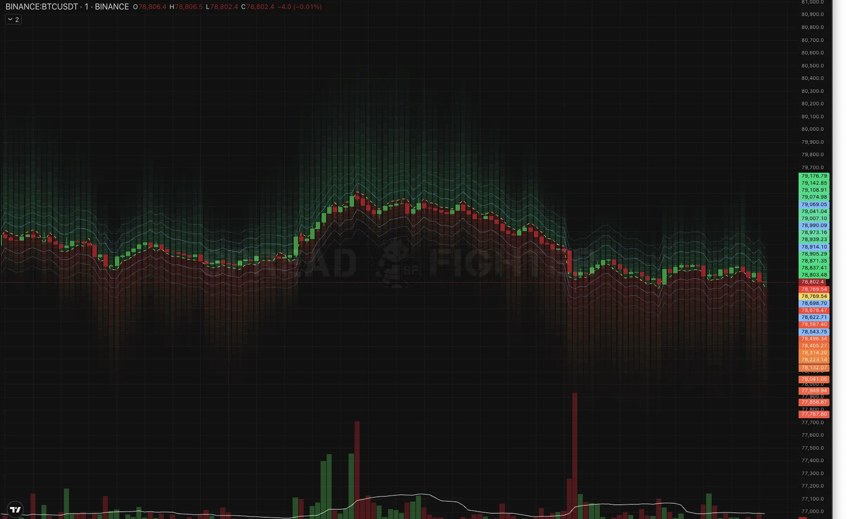
The map over BTCUSDT candles: a red zone of long wipe-outs below, a green zone of short wipe-outs above, a yellow dashed line at the center, and blue lines for the stop-out probability.
What it is
Liquidation Map is an indicator drawn over the candles, not in a separate pane. Instead of lines, it shows a continuous heatmap: red downward for the zone where long positions get wiped out, green upward for the zone where shorts get wiped out.
All numbers below come from running the model forward month by month over 9.5 months of Binance USDT-M history. The main slice is 20 instruments and three folds (March, June, September 2026), with a 60-minute horizon. The unit of observation is an instrument×fold cell, so stability is visible and not hidden in an average. Acceptance was extended to 433 instruments and 1,267 cells.
The stripes are not levels
This is the most expensive reading mistake, so let's remove it first. The horizontal stripes inside the map are not a set of levels with something standing behind each one. They are a single continuous density, cut into rows only so that it can be drawn. The third row has no meaning different from the fourth.
Moreover, the row grid changes from bar to bar: the rows split the width of the band itself, not percentages of price. Holding on to a specific row means holding on to a drawing artifact.
Why not lines. The very same map, shown as six lines at density quantiles, captures 5.5 pp less liquidation volume than having no prediction at all. The heatmap on the same data captures 12.3 pp more.
The reason is geometric. With asymmetry, the side where the model expects volume gets wider. The heatmap spends more area on it, so attention goes where a move is expected. Quantile lines do the opposite: the wider the side, the farther its lines move from price, while liquidations cluster near price.
What matters is the band boundary, the outer edge of the colored zone on your side. Separately, there are the blue risk lines, which have their own scale and meaning, described below. Everything else inside the map is a gradient, read by eye and not by divisions.
How to read the picture
| Element | What it means |
|---|---|
| Red below | Zone where longs get wiped out. The brighter it is, the denser the expected volume of forced selling there |
| Green above | Zone where shorts get wiped out. The color follows who gets wiped out, not the side of the order book |
| Yellow dashed | Map center. Its offset from price is the predicted side of the flow |
| Blue dashed | Risk lines: the probability that price gets carried to this point within the horizon. They are symmetric around price, unlike the map |
The sides are deliberately of different widths, and the asymmetry is the main thing the map tells you. The width of a side already contains the probability: if the model expects volume down, the red side is wider than the green one. Brightness does not duplicate this.
Stop distance — confirmed
+0.128 to the stop-out rate inside the band · 121 cells out of 121
This is the most solid result of the whole study and the main reason to open the indicator. The stop-out rate by candle lows inside the band is 0.128 higher than at the same distance beyond it, at a matched σ-distance, so the comparison is not bought by volatility. It is unanimous: 121 instrument×fold cells out of 121.
It reads literally: a stop inside the colored zone gets taken out noticeably more often than at the same distance but beyond its edge. Place it beyond the outer edge of the hot zone on your side.
If the band is wider than you are willing to tolerate, that is not a reason to move the stop inside it. It is a reason to reduce position size or skip the entry.
To calibrate expectations, here is the median effective distance of liquidated positions from entry:
| Instruments | Distance |
|---|---|
| BTC, ETH | 0.48% |
| Altcoins | 1.1 – 1.9% |
Stop-out risk lines
The band answers where volume will settle. The risk lines answer a different question: how often price gets carried to that place at all. These are two different quantities, and they cannot be shown in one channel: the map's color is already taken by density, and the +12.31 pp was measured on exactly this geometry.
The probability of reaching a level is computed with the reflection principle: p = 2(1 − Φ(d / σ√h)). The "25%" line reads literally: a stop on it gets taken out in about a quarter of cases within the horizon. There are three pairs by default: 50, 25 and 10 percent, and the values are configurable.
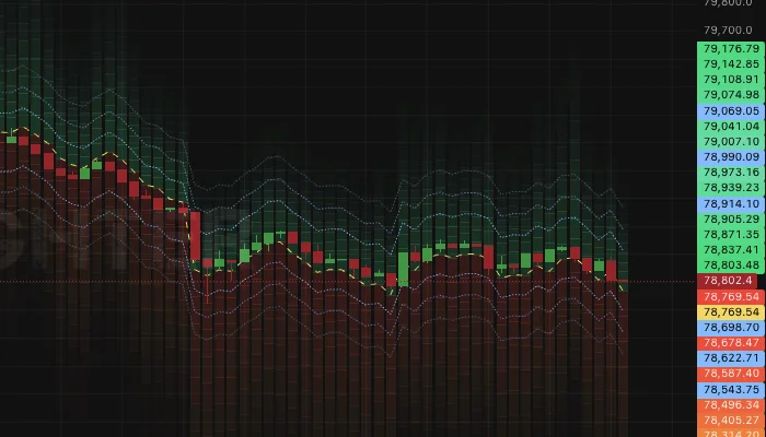
Risk lines over the heatmap. They are symmetric around price, the map is not.
The symmetry is not an oversight. The probability of reaching a level depends on distance and volatility, but not on which side is hotter. The hypothesis "the side adds to the stop-out probability" was tested at fixed width and not confirmed. That is why these are two different objects on the chart, and the lines are cold-colored: red and green already mean the side of the wipe-out.
This also removes the objection to levels in general. What was rejected were lines at density quantiles: that quantity is not monotonic, and a "third level" is arbitrary. The probability of reaching a level is monotonic in distance, so levels are legitimate here.
The whole rule: place the stop beyond the outer edge of the colored zone and farther than the risk line you are willing to tolerate. The first is a measured correction on top of distance, the second is the distance itself.
Where fuel has built up — confirmed
+12.31 pp on 20 instruments (59 of 60) · +9.84 pp on 433 (1058 of 1267)
Hot bins capture 12.31 pp more of the next hour's liquidation volume than a band of the same width and the same number of bins, but without a prediction. The gain cannot be bought with width, because width is equalized by construction.
In practice: the bright zone is fuel. If price reaches it, the move is likely to accelerate and not fade. It works as a place for partial profit-taking along the move, and as an explanation of why a breakout right here went in a jerk.
A fair expectation is about ten points on a typical instrument, not fifteen. On the broad universe the 10th percentile is −3.21 pp, meaning one cell in ten has a negative result; the 90th is +22.70.
Side when choosing a stop — not confirmed
+0.009 at fixed width · 69 cells out of 135
The hypothesis was this: a stop on the model's "hot" side gets taken out more often than on the cold one. With a fair control, comparing the model's hot bins against the cold ones within the set of the null map's hot bins, that is, at fixed width, what remains is +0.009 and 69 cells out of 135. That is noise.
Takeaway for your work: when choosing stop distance, rely on width, not on which side you are on.
Price direction — refuted
spread of the extreme deciles −3.84 bp with a standard error of the difference 8.52 · t = −0.45
The map does not show where price will go. Average return over the horizon by deciles of the predicted side is non-monotonic, and the difference between the extreme deciles is indistinguishable from zero.
The fact that the red side is wider means "if the move happens down, this many longs will be wiped out", not "it will go down". Entering by the side of the map is a mistake, and this was measured, not assumed.
The side of the flow is quite predictable on its own (AUC 0.69 on the hourly horizon, volume accuracy 78% against 64% for the instrument's constant), but this is a prediction about who gets wiped out, not about where price goes. The difference is not formal: liquidations happen where price goes, not the other way around.
When to trust the map more
The map's main lever is shifting width to the predicted side. If the real flow is symmetric, there is nothing to redistribute, and any asymmetry will be wrong in half of the cases. Hence a direct dependence.
Effect by quartiles of flow one-sidedness, September 2026:
| Long share of the liquidation flow | Instr. | Effect | Positive |
|---|---|---|---|
| 0.10 – 0.61 — balanced | 108 | +3.47 | 76 / 108 |
| 0.62 – 0.78 | 108 | +5.62 | 83 / 108 |
| 0.78 – 0.86 | 108 | +8.06 | 93 / 108 |
| 0.86 – 1.00 — most one-sided | 109 | +10.11 | 97 / 109 |
The correlation is +0.294. In trending and cascading periods the map gives ten points and more, in a range three or four. For an indicator this is a favorable dependence: the effect is larger where it is needed more.
Thin instruments work better than liquid ones, counter to intuition. By quintiles of the number of half-hour windows with liquidations, the thinnest give +9.9 and +18.7 in March and June, the most liquid +7.0 and +10.1. The explanation is mechanical: on very liquid instruments liquidations are spread more evenly across price, and there is little to focus attention on.
Settings
The width of the map grows as the square root of the horizon. On an hourly horizon sigma is on the order of one percent, and on a one-minute chart such a band is wider than price moves across the whole screen: the map degenerates into a solid slab, because within one sigma the Gaussian barely decays. That is why you pick the horizon to match the timeframe.
| Chart timeframe | Horizon | What you see |
|---|---|---|
| 1m | 15 min | The whole gradient, axis not stretched |
| 5 – 15m | 60 min | The main slice of the study |
| 1h and higher | 240 min | A wide band for a wide bar |
- Span, sigmas — how many sigmas of density to draw. 2.5 by default; beyond that the density falls below five percent of the peak.
- Max distance from price, % — a display limit, not a model limit. It trims only the drawing, so that autoscale doesn't stretch the axis and flatten the candles. 1.5 by default.
- Stop-out risk 1, 2, 3, % — the probabilities for which the blue lines are drawn. 50, 25 and 10 by default.
- Lower sigma and Upper sigma — two lines for the map boundary, off by default. Turn them on if you need an explicit edge instead of a gradient.
What the map does not include
The strongest part of the model for timing is not shown in the map itself: the intensity and the cascade regime. It lives in a separate screener: Liquidation Spike.
The reason for the split is substantive, not technical. The map answers "where" for a single instrument, while intensity answers "where and when" across the whole market at once. Measured: a minute with ten or more visible liquidations gives a volume over the next five minutes 9.7 times above the seasonal base, over fifteen 6.1 times, over an hour 3.6 times. The probability of an event in the next five minutes is 86%. 92% of the volume of the next fifteen minutes falls on the side of the spike — 7 folds out of 7, 20 instruments out of 20.
But price pulls back anyway: the move continues in 44% of cases, and with thirty or more liquidations in a minute only in 17%. So a cascade is a strong signal about timing and the side of the flow, and again not about price direction.
The workflow: the spike screener finds the instrument, and the map on its chart gives the stop distance. Neither gives direction.
The map is computed once a minute on a closed candle, from one-minute candles and the stream of forced liquidations. Open interest, funding, basis and the order book are not included: their contribution was tested on correctly built maps and is indistinguishable from zero. The same model, accumulated on a fixed price grid, is Liquidation Heatmap.