SF - Common active return measure
A classic risk management model that compares expected return, benchmark return, and risk-free return.
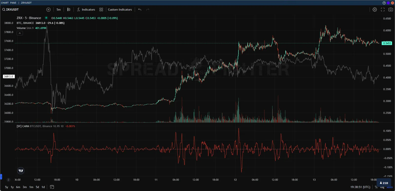
Functionality
The indicator is an oscillator with a percentage scale and has the following settings:
- Benchmark ticker - the symbol of the benchmark instrument (BTC by default);
- Risk free rate - the annual risk-free rate in percent (10.95% by default, the average return of a funding rate payment arbitrage strategy);
- Length - the oscillator length.

User parameters
In the style settings window, the user can choose the display colors and the transparency of the indicator.

Indicator style settings
Access by plan
The indicator is available on all subscription versions.
Model description
The model (CAPM) describes the relationship between systematic risk, or overall investment risk, and the expected return of assets. It is a financial model that sets a linear relationship between the required return on an investment and risk. The model is based on the relationship between an asset's beta coefficient, the risk-free rate (usually the return of a funding rate arbitrage strategy), and the equity risk premium, or the expected market return minus the risk-free rate.
CAPM developed as a way to measure this systematic risk. It is widely used in finance to price risky securities and to derive the expected return of assets given their risk and the cost of capital.
CAR calculation
The formula for the expected return of an asset, given its risk, is:
where is the expected return of the asset, is the risk-free rate, is the beta coefficient, and is the market risk premium.
So asset holders expect compensation for risk and for the time value of money. The risk-free rate in the CAPM formula accounts for the time value of money. The other components of the CAPM formula account for the investor taking on extra risk.
The purpose of the CAPM model is to assess whether a stock is fairly valued when its risk and the time value of money are compared with its expected return. In other words, if you know the individual parts of CAPM, you can judge whether the stock's current price matches its likely return.
CAPM, CARM, and the Beta coefficient (β)
An asset's Beta coefficient (β) measures how much risk the asset adds to a portfolio relative to the broad market or the benchmark return. If an asset is riskier than the market, its beta is greater than one. If an asset has a beta below one, the formula implies it will reduce the risk of the portfolio.
The asset's beta is then multiplied by the market risk premium, which is the return expected from the market above the risk-free rate. Then the risk-free rate is added to the product of the asset's beta and the market risk premium. The result should give the investor the required return, or discount rate, that they can use to determine the value of the asset.
CARM (common active return measure) is effectively the beta coefficient in CAPM calculations. It reflects the sensitivity of the asset's equity relative to the benchmark.
CAPM example - a portfolio that beats the market
Ticker: BLZUSDT*16103.06+OCEANUSDT*6849.32+TOMOUSDT*3174.6+TRBUSDT*86.89
To keep things simple, assume the agent invested $ 1000 in each project. The positions as of 10 Nov 2022 are then:
| Asset | Price | Position | Symbol |
|---|---|---|---|
| BLZ | $ 0.0621 | $ 1000 / $ 0.0621 ~ 16103.06 | BLZUSDT*16103.06 |
| OCEAN | $ 0.1460 | $ 1000 / $ 0.1460 ~ 6849.32 | OCEANUSDT*6849.32 |
| TOMO | $ 0.315 | $ 1000 / $ 0.315 ~ 3174.6 | TOMOUSDT*3174.6 |
| TRB | $ 11.51 | $ 1000 / $ 11.51 ~ 86.89 | TRBUSDT*86.89 |
In this case, the agent's portfolio beats the benchmark by ~300%. CARM stays strictly in the positive zone.
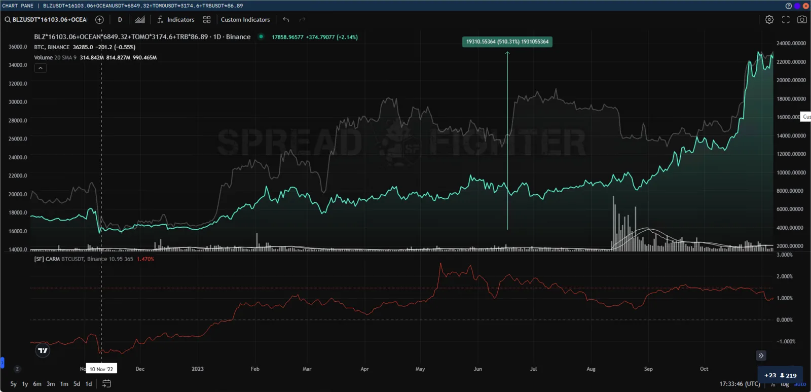
A portfolio that beats the market
CAPM example - a portfolio that lags the market
Ticker: GMTUSDT*2388.35+REEFUSDT*253936.01+RSRUSDT*219780.22+SUSHIUSDT*797.45
The positions as of 10 Nov 2022 are:
| Asset | Price | Position | Symbol |
|---|---|---|---|
| GMT | $ 0.2367 | $ 1000 / $ 0.2367 ~ 2388.35 | GMTUSDT*2388.35 |
| REEF | $ 0.003938 | $ 1000 / $ 0.003938 ~ 253936.01 | REEFUSDT*253936.01 |
| RSR | $ 0.00455 | $ 1000 / $ 0.00455 ~ 219780.22 | RSRUSDT*219780.22 |
| SUSHI | $ 1.254 | $ 1000 / $ 1.254 ~ 797.45 | SUSHIUSDT*797.45 |
In this case, the agent's portfolio lags the benchmark by ~60%. CARM stays strictly in the negative zone.
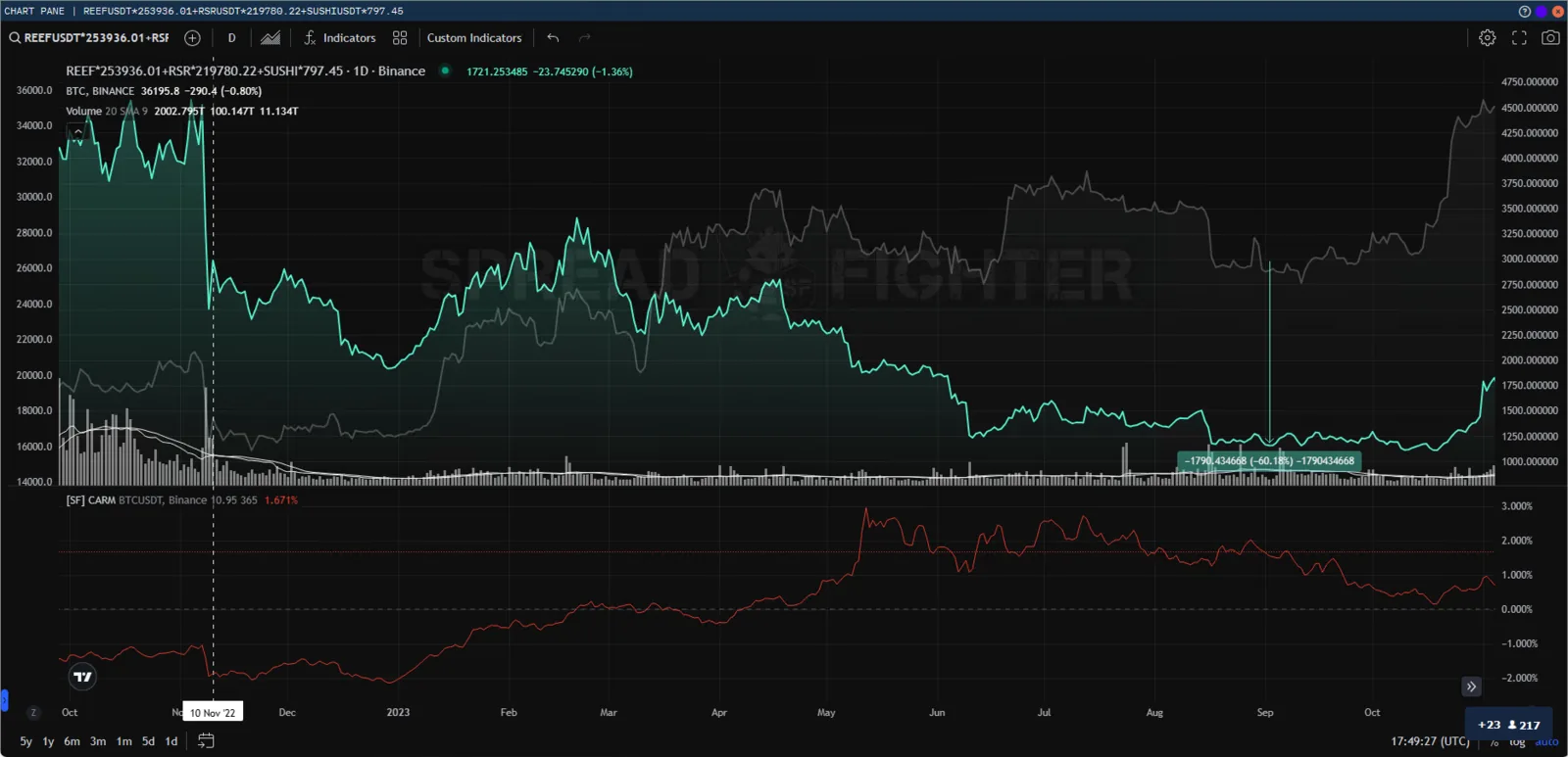
A portfolio that lags the market
CAPM example - the market portfolio
In this case, the CARM value is zero.
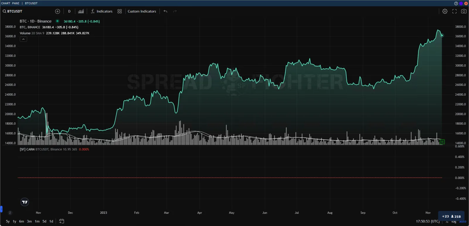
The market portfolio
Problems with CAPM
Unrealistic forecasts
Some assumptions behind the CAPM formula do not hold in reality. Modern financial theory rests on two postulates:
- Securities markets are highly competitive and efficient (that is, relevant information about assets spreads quickly and everywhere and is reflected in prices).
- These markets are dominated by rational, risk-averse investors who seek to maximize the returns on their investments.
As a result, it is not entirely clear whether CAPM works. The beta coefficient is a major stumbling block.
When professors Eugene Fama and Kenneth French studied stock returns on the New York Stock Exchange, the American Stock Exchange, and Nasdaq, they found that differences in beta coefficients over a long period do not explain the performance of different stocks. The linear relationship between beta and the returns of individual stocks also breaks down over shorter periods. These results seem to suggest that CAPM may be flawed.
Including the beta coefficient in the formula assumes that risk can be measured by the volatility of stock prices. However, price moves in the two directions are not equally risky.
CAPM also assumes that the risk-free rate stays constant over the discounting period.
Suppose, in the previous example of professors Eugene Fama and Kenneth French, that the interest rate on US Treasury bonds rose to 5% or 6% during a 10-year holding period. A higher risk-free rate also raises the cost of capital used in investments and can make stocks look overvalued.
Estimating the risk premium
The market portfolio used to determine the market risk premium is only a theoretical quantity. It is not an asset you can buy or invest in as an alternative. Most of the time, investors will use a benchmark as a substitute for the market, which is an imperfect comparison.
The most serious criticism of CAPM is the assumption that future cash flows can be estimated for the discounting process. If an investor could estimate future stock returns with a high degree of accuracy, CAPM would not be needed.
CAPM and the efficient frontier
Using CAPM to build a portfolio is supposed to help the investor manage risk. If an investor could use CAPM to optimize portfolio return against risk perfectly, they would sit on a curve called the efficient frontier, shown in the following chart.
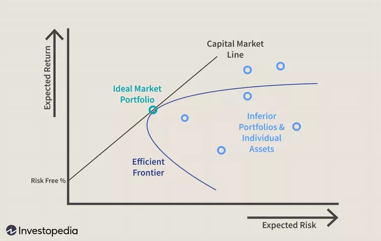
Efficient frontier curve
The chart shows how a higher expected return (Y axis) requires more expected risk (X axis). Modern portfolio theory holds that, starting from the risk-free rate, the expected return of a portfolio grows as risk grows. Any portfolio that lies on the capital market line (CML), is better than any possible portfolio to the right of that line, but at some point a theoretical portfolio can be built on the CML with the best return for the amount of risk taken.
The CML and the efficient frontier can be hard to determine, but they illustrate an important concept for investors: there is a trade-off between higher return and higher risk. Because it is impossible to build a portfolio that matches the CML perfectly, investors more often take on too much risk in pursuit of extra profit.
The next diagram shows two portfolios that were built to lie on the efficient frontier. Portfolio A is expected to return 8% a year and has a standard deviation, or risk level, of 10%. Portfolio B is expected to return 10% a year, but its standard deviation is 16%. The risk of portfolio B grew faster than its expected return.
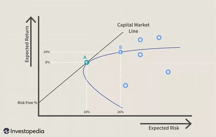
Comparing portfolios A and B
The practical value of CAPM
Given the criticism of CAPM and the assumptions behind using it to build a portfolio, it can be hard to see how it can be useful. Still, CAPM can have some value as a tool for testing whether future expectations are reasonable or for making comparisons.
Imagine an adviser who suggested adding a stock priced at 100 dollars to a portfolio. The adviser uses CAPM to justify the price with a 13% discount rate. The adviser's investment manager can take this information and compare it with the past performance of the company and its peers to see whether a 13% return expectation is reasonable. Suppose in this example that the return of the comparable group over the last few years was just above 10%, while this stock consistently lagged with a 9% return. The investment manager should not accept the adviser's recommendation without some justification for the higher expected return.
An investor can also use the concepts of CAPM and the efficient frontier to evaluate the performance of their portfolio or of individual stocks against the rest of the market. For example, suppose an investor's portfolio earned 10% a year over the last three years, with a standard deviation of returns (risk) of 10%. Over the same three years, however, the average market delivered a 10% return at 8% risk.
The investor can use this observation to re-evaluate the structure of their portfolio. It could explain why the investor's portfolio sits to the right of the CML. If you can identify assets that either reduce return or disproportionately raise the portfolio's risk, the investor can make changes to improve return. Unsurprisingly, CAPM has contributed to the growth of indexing, or building a stock portfolio to mimic a given market or asset class, by risk-averse investors. This is largely because of the CAPM message that you can earn a higher return than the market as a whole only by taking on higher risk (beta).
Who came up with CAPM?
The CAPM model was developed in the early 1960s by the financial economists William Sharpe, Jack Treynor, John Lintner, and Jan Mossin, who built on ideas put forward by Harry Markowitz in the 1950s.
What assumptions does the CAPM model make?
These are the assumptions made in the CAPM model:
- All investors are risk-averse by nature.
- Investors have the same time horizon for evaluating information.
- There is unlimited capital that can be borrowed at the risk-free rate of return.
- Investments can be divided into an unlimited number of parts and sizes.
- There are no taxes, inflation, or transaction costs.
- Risk and return are linearly related
Many of these assumptions have been challenged as unrealistic or simply wrong.
What are some alternatives to CAPM?
Because of the criticism of the CAPM model, several alternative models have been developed to understand the relationship between risk and reward in investing.
One of them is arbitrage pricing theory (APT), a multifactor model that considers many factors grouped into macroeconomic or sector-specific factors.
Another option is the Fama-French three-factor model, which extends the CAPM model by adding value risk factors to market risk factors.
What is the International Capital Asset Pricing Model (ICAPM)?
The International capital asset pricing model (ICAPM) is a financial model that applies the traditional CAPM principle to international investments. It extends CAPM by accounting for the direct and indirect effect of foreign currency, in addition to the time value and market risk included in CAPM.
Key takeaways
CAPM uses the principles of modern portfolio theory to determine whether an asset is fairly valued. It relies on assumptions about investor behavior, the distribution of risk and return, and market fundamentals that do not hold in reality. Still, the basic concepts of CAPM and the related efficient frontier can help investors understand the relationship between expected risk and reward, as they try to make better-informed decisions about adding assets to a portfolio.
- The CAPM model is a financial model that calculates the expected rate of return for an asset.
- CAPM does this using the expected return of both the market and a risk-free asset, as well as the asset's correlation or sensitivity to the market (beta).
- CAPM has some limitations, such as unrealistic assumptions and a linear interpretation of the risk-return relationship.
- Despite its problems, the CAPM formula is widely used because it is simple and makes it easy to compare investment alternatives.
- For example, CAPM is used together with modern portfolio theory to understand portfolio risk and expected return.
Source: investopedia