Realized volatility, Local volatility, GARCHM, AGARCH, APGARCH volatility, CEV, IK, Hull-White volatility model, Normalized average true range volalility

Various volatility models.

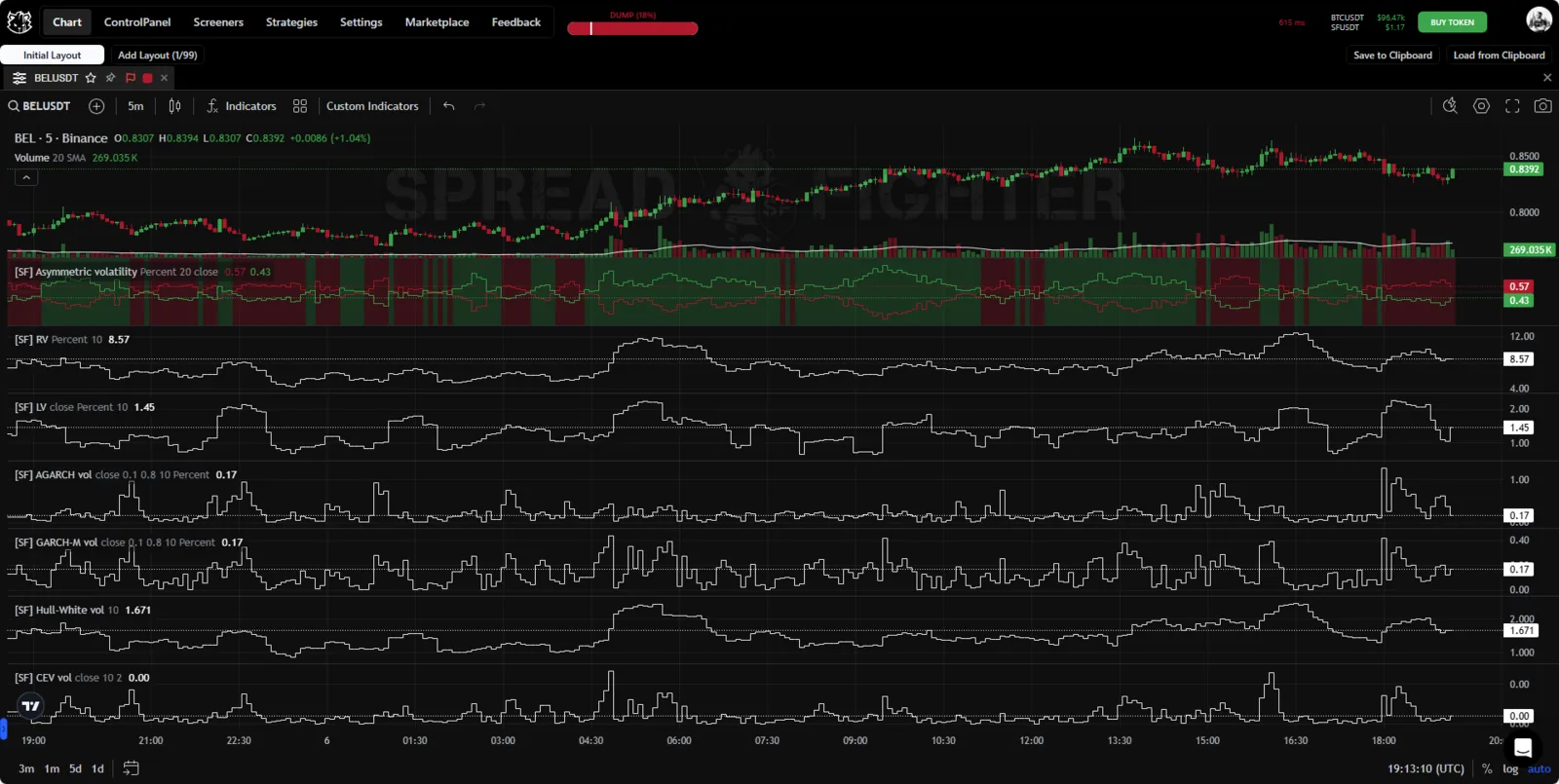
Indicator appearance.

Description

Realized volatility

Realized volatility (RV) sums the price range in which the price moved over a given period of time. Realized volatility is calculated by the formula:

$$RV_x = \sum_{i=0}^{x}(high_i-low_i)$$

where $high$ is the bar high, $low$ is the bar low, and $x$ is the given period of time.

Local volatility

The traditional volatility calculation involves computing the standard deviation of returns, which is based on the mean return. However, when an asset's price shows a trending move, the mean return can differ significantly from zero, and changing the length of the time window used for the calculation can produce artificially inflated volatility values. To solve this problem, the local volatility model was developed. It calculates the standard deviation of the differences between consecutive asset prices, not of their returns. This shows how much the price changes from one tick to the next, regardless of the overall trend.

GARCH-M

The GARCH model (generalized autoregressive conditional heteroskedasticity) is a statistical model used to forecast the volatility of a financial asset. The model accounts for fluctuations in volatility over time, recognizing that volatility can change in a heteroskedastic way (that is, with non-constant variance) and can be influenced by past events.

The main advantage of GARCH models is their ability to model volatility as changing over time, which makes them especially suitable for analyzing financial markets, where volatility is not constant. In GARCH models, volatility at a given moment depends both on past values of volatility itself and on past shocks (innovations) in the data. This lets the models account for conditional heteroskedasticity, a phenomenon where the distribution of a variable is unstable over time.

GARCH-in-Mean (GARCH-M) was proposed by Engle et al. in 1987. It is not a special model for conditional variance. It is about using conditional variance as one of the factors of a regression model for the risk premium.

General formula of the GARCH-M model:

$$y_{t}= α + f(σ^2_t) - E|f(σ^2_{t+1})| + u_t$$

where:

$σ^2_{t}$ is the conditional variance at time $t$ (that is, squared volatility), and $α$ is the coefficient representing the effect of the squared lagged error on the conditional variance.

In the context of financial forecasting, the GARCH model is used to estimate the future volatility of an asset.

AGARCH

The AGARCH model is an extension of the standard GARCH (Generalized Autoregressive Conditional Heteroskedasticity) model. It was proposed to better account for asymmetry and the leverage effect inherent in many financial series (the influence of market leverage on asset volatility). The leverage effect is that negative returns (losses) usually lead to higher volatility than positive returns (profits) of the same size.

The AGARCH model is useful in financial modeling for estimating asset volatility that accounts for asymmetry and leverage effects. It is widely used to estimate market risks, in structuring financial products, and in research on finance and econometrics.

The AGARCH model is calculated by the formula:

$$σ^2_t = α_0 + \sum^q_{i=1}{α_i(u_{t-i}-γ)^2}+\sum^p_{j=1}β_jσ^2_{t-j}$$

where: $σ^2_t$ is the conditional variance (volatility) at time t, and $\alpha$, $\gamma$ and $\beta$ are non-negative model parameters,

Note that in real conditions, the most accurate estimates of volatility and risk may require adapting the model, for example by extending it to AGARCH with more lags for both volatility itself and the innovations. These extensions let you tune the model more finely to the specifics of the data and reach more accurate forecasts.

Constant Elasticity of Variance

The constant elasticity of variance (CEV) volatility model assumes that an asset's volatility changes depending on its price level. The CEV model is commonly used in financial mathematics and in option analysis.

$$dS_t = μ S_t dt + \sum{S_t^{β} dW_t}$$

Hull-White volatility model

The Hull and White volatility model, presented in their 1987 papers, is a development of the standard Black-Scholes option pricing model. It aims to account for and model the volatility of the underlying asset over time more accurately, which makes it especially important for financial analysis and option valuation.

The Black-Scholes model assumes that an asset's volatility is a constant, which is far from always true. Hull and White proposed using local volatility, which can change over time while remaining a deterministic function of the current asset price and time. This made it possible to reflect the real behavior of prices in financial markets more accurately and to give more accurate option values.

The core of the model is applying stochastic calculus techniques to model the price dynamics of the underlying asset with variable volatility. In the Hull-White model, the analyzed volatility of the underlying asset changes with time and the asset price level, which allows a more flexible approach to risk management and pricing of derivative financial instruments.

$$r_t=k_t(θ_t-r_t)dt+σ_tdW_t$$

where $θ_t=f(0,t)+\dfrac{ð_tf(0,t)}{k_t}+\dfrac{1}{k_t}\int^t_0 σ^2_ue^{-2\int^u_0k_sds}du$ is the conditional variance (volatility).

tip

Disclaimer: It is important to understand that this indicator does not reflect the real CEV model with all its mathematical details. It is intended only for a qualitative assessment of changes in volatility. The exact mathematical expression of a stochastic volatility model can vary with the modifications and additions researchers make to adapt the model to specific tasks and market conditions.

Normalized average true range volalility

The normalized average true range (NATR) volatility indicator is a tool designed to measure market volatility by normalizing the average true range (ATR) relative to the price level. NATR is calculated by the formula:

$$NATR = \dfrac{1}{n} \times \sum^{(n)}_{i=1}{(high_i - low_i)} \times \dfrac{1}{hlc3} \times 100$$

where $high$ is the bar high, $low$ is the bar low, $hlc3$ is the typical price, and $x$ is the given period of time.

Asymmetric volatility

The asymmetric volatility model measures the difference between the upward and downward volatility of an asset's price, using dynamic McGinley smoothing and an optional volatility clustering correction.

First, the directional moves are calculated.

$$U_t = \max(C_t - C_{t-1}, 0)$$ $$D_t = \max(C_{t-1} - C_t, 0)$$

where: $U_t$ is the upward price move on bar $t$, $D_t$ is the downward price move on bar $t$, and $C_t$ is the closing price on bar $t$.

The total absolute volatility over the period $n$ is calculated.

$$T_t = \sum_{i=0}^{n-1} |C_{t-i} - C_{t-i-1}|$$

where $T_t$ is the sum of the absolute price changes over the last $n$ bars.

The averaged directional volatility is calculated:

$$UV_t = \frac{\sum_{i=0}^{n-1} U_{t-i}}{n}$$ $$DV_t = \frac{\sum_{i=0}^{n-1} D_{t-i}}{n}$$

where: $UV_t$ is the average upward directional volatility, and $DV_t$ is the average downward directional volatility.

If normalization (in percent) is selected, the following is applied:

$$UV^{prc}_t = \frac{UV_t}{T_t} \times 20$$ $$DV^{prc}_t = \frac{DV_t}{T_t} \times 20$$

McGinley smoothing is calculated by the formula:

$$MD_t = MD_{t-1} + \frac{C_t - MD_{t-1}}{\min(P, \max(1, k \cdot P \cdot (\frac{C_t}{MD_{t-1}})^e))}$$

where: $MD_t$ is the smoothed value, $P$ is the smoothing period length, $k$ is the smoothing coefficient (usually 0.6), and $e$ is the exponent (usually 2.0).

McGinley is applied separately to upward and downward volatility:

$$UV^{MG}_t = MD(UV_t)$$ $$DV^{MG}_t = MD(DV_t)$$

The volatility clustering correction is performed:

$$VPerf_t = EMA(|C_t - C_{t-1}|, \text{cluster period})$$

Adjustment factor:

$$AF_t = \max(f, 1 - \frac{VPerf_t}{100})$$

where: $f$ is the clustering coefficient (usually 0.85), and $AF_t$ is the adjustment factor.

Applying the adjustment:

$$UV^{Adj}_t = UV^{MG}_t \times AF_t$$ $$DV^{Adj}_t = DV^{MG}_t \times AF_t$$

Local volatility (LV): what it is and how it works

What is local volatility (LV)?

Local volatility (LV) is a volatility measure used in quantitative analysis. It helps give a fuller picture of volatility by taking into account both strike prices and time to derive price and risk statistics. Local volatility is related to an option's implied volatility and can be extrapolated from it.

Understanding local volatility

The concept of local volatility was introduced by economists Emanuel Derman and Iraj Kani. Local volatility tries to determine the actual volatility of an asset across a range of strike prices. Local volatility uses two-factor analysis to give more accurate actual volatility readings than implied volatility. When plotted, local volatility usually fits the data better than implied volatility. Some scholars believe that although implied volatility can be used to get the right price, local volatility is, from a logical point of view, a more suitable input.

Local volatility essentially replaces the constant volatility function that is calculated from the strike price. Instead, local volatility answers the same risk question differently, by looking at the asset price and time, which gives a different view of volatility from the same inputs.

Because local volatility is often extrapolated from implied volatility, it is sensitive to changes in implied volatility. This means small changes in implied volatility lead to sharper changes in local volatility.

How local volatility is used

One of the main criticisms of the original Black-Scholes model is that it tried to fix the volatility of the underlying asset at a constant level over the whole life of the option. This does not reflect the actual market data we have, but the model is still one of the most effective option pricing schemes.

Local volatility can be especially useful when pricing exotic options, which are hard to fit with standard models. It is designed to match market prices and can be used to price all combinations of strikes and maturities, as opposed to a single maturity that implied volatility covers.

Still, both local and implied volatility are often studied together and compared with historical volatility. While local and implied volatility are generated from current price levels using the Black-Scholes model, historical volatility can be used to produce a Black-Scholes model price that is adjusted by past data on actual price movements.

Source: investopdeia

The GARCH model: definition and use in statistics

What is generalized autoregressive conditional heteroskedasticity (GARCH)?

Generalized autoregressive conditional heteroskedasticity (GARCH) is a statistical model used in analyzing time series data, where the error variance is believed to be serially autocorrelated. GARCH models assume that the variance of the error term follows an autoregressive moving average process.

Understanding generalized autoregressive conditional heteroskedasticity (GARCH)

Although GARCH models can be used to analyze a number of different types of financial data, such as macroeconomic data, financial institutions usually use them to estimate the volatility of returns on stocks, bonds and market indexes. They use the resulting information to set prices and judge which assets will potentially bring higher returns, and to forecast the returns of current investments, to help with asset allocation, hedging, risk management and portfolio optimization decisions.

GARCH models are used when the error variance is not constant. That is, the error term is heteroskedastic. Heteroskedasticity describes the irregular pattern of variation of an error term or variable in a statistical model.

Essentially, wherever there is heteroskedasticity, observations do not follow a linear pattern. Instead, they tend to cluster. Therefore, if statistical models that assume constant variance are applied to this data, the conclusions and predictive value you can draw from the model will not be reliable.

The error variance in GARCH models is assumed to vary systematically, depending on the average size of the error in previous periods. In other words, it has conditional heteroskedasticity, and the reason for the heteroskedasticity is that the error term follows an autoregressive moving average model. This means it is a function of the average of its own past values.

History of GARCH

GARCH was developed in 1986 by Dr. Tim Bollerslev, then a graduate student, as a way to solve the problem of forecasting asset price volatility. It is based on economist Robert Engle's groundbreaking 1982 work introducing the autoregressive conditional heteroskedasticity (ARCH) model. His model assumed that the variation of financial returns is not constant over time, but is autocorrelated, or conditional on or dependent on each other. For example, this can be seen in stock returns, where periods of return volatility tend to cluster together.

Since it first appeared, many variations of GARCH have emerged. They include the nonlinear one (NGARCH), which accounts for correlation and the observed "volatility clustering" of returns, and integrated GARCH (IGARCH), which constrains the volatility parameter. All variants of the GARCH model seek to account for the direction, positive or negative, of returns in addition to the magnitude accounted for in the original model.

Each GARCH derivation can be used to account for the specific qualities of a stock, an industry or economic data. When assessing risk, financial institutions include GARCH models in their risk premium and in their maximum expected loss (whether for a single investment or trading position, a portfolio, or at the level of a division or the whole firm) over a given period of time. GARCH models are considered to give more accurate risk measurements than those obtained by tracking only the standard deviation.

Various studies have been carried out on the reliability of different GARCH models in different market conditions, including in the periods before and after the Great Recession.

Source: investopedia